Handling OTU Tables in Python

I have recently been working a lot with OTU tables in the BIOM (Biological Observation Matrix) format, generated by QIIME and PIPITS. This now-common OTU table format seems to be getting more popular; I don’t recall running into such files in my bioinformatics studies just a few years back.

Tool suites like QIIME allow you to treat BIOM-formatted OTU tables as black boxes, keeping the users insulated from their internals, but I wanted to examine them a bit in Python. They are HDF-formatted files, version 5 in recent tools. Installing the h5py package along with the ancillary tables package seems to be a good way to go, but does not work. The tables package does not handle variable length strings.

The easiest way to inspect OTU tables in Python is with the biom-format package, which interestingly uses the h5py package that I could not get to work.

For starters, installation:

pip install biom-format
pip install h5py
pip install pandas
pip install numpy

And now a tour through a sample OTU table. The biom-format documentation didn’t make it obvious how to open an BIOM file, but it turns out that they provide a load_table routine that accepts a filename. There is a ‘sample’ axis and an ‘observation’ axis, where the observations are the OTUs.

>>> from biom import load_table
>>> t = load_table(‘sample_otu_table.biom')
>>> print(t.ids())
['SA8' 'Bed' '26' '29' 'Food' 'CA4' '5' 'SA3' 'Water' '15' '22' 'SA15'
 'SA25' 'CA22' '1' 'TRI3' '24' '10' '14' 'PA36' '3' '7' '16' '21' 'PA17'
 'CA8' '25' 'PA60' 'PA29' 'PA71' 'PA53' 'PA79' 'PA64' 'PA46' 'PA6' 'TRI18'
 'TRI8' '8' 'CA17' 'PA1' '13' '27' '11' '28' '9' '4' '2' '18' '12' '23'
 'PA19' 'HydroGel' '6' '20' '30' '19' 'TRI24' '17']
>>> print(t.ids(axis='observation'))
['4371191' '4479944' '816470' ... '512148' '1109141' '3275744']
>>> print(t.data('SA8', axis='sample'))
[2. 0. 0. ... 0. 0. 0.]
>>> print(t.data('4371191', axis='observation'))
[2. 5. 1. 1. 1. 0. 0. 0. 0. 0. 0. 0. 0. 0. 0. 0. 0. 0. 0. 0. 0. 0. 0. 0.
 0. 0. 0. 0. 0. 0. 0. 0. 0. 0. 0. 0. 0. 0. 0. 0. 0. 0. 0. 0. 0. 0. 0. 0.
 0. 0. 0. 0. 0. 0. 0. 0. 0. 0.]

The taxonomy metadata annotations are easily available, allowing one to quickly access a list of all taxa present in the study.

>>> print(t.metadata('4371191', axis='observation')['taxonomy'])
['k__Bacteria', 'p__Proteobacteria', 'c__Gammaproteobacteria', 'o__Pseudomonadales', 'f__Pseudomonadaceae', 'g__Pseudomonas', 's__']
>>> metadata_df = t.metadata_to_dataframe('observation')
>>> metadata_df.columns = ['kingdom', 'phylum', 'class', 'order', 'family', 'genus', 'species']
>>> print(metadata_df.head())
 kingdom phylum class \
4371191 k__Bacteria p__Proteobacteria c__Gammaproteobacteria
4479944 k__Bacteria p__Actinobacteria c__MB-A2-108
816470 k__Bacteria p__Firmicutes c__Bacilli
842143 k__Bacteria p__Actinobacteria c__Actinobacteria
99682 k__Bacteria p__Proteobacteria c__Gammaproteobacteria

order family genus species
4371191 o__Pseudomonadales f__Pseudomonadaceae g__Pseudomonas s__
4479944 o__0319-7L14 f__ g__ s__
816470 o__Bacillales f__Bacillaceae g__ s__
842143 o__Actinomycetales f__Cellulomonadaceae g__Cellulomonas s__
99682 o__Pseudomonadales f__Pseudomonadaceae g__Pseudomonas s__

Methods are provided to collapse the table over particular levels of taxonomy, to normalize the data across samples to account for difference in sampling depth, and many other useful operations. (This code was borrowed from the biom-format documentation.)

>>> phylum_idx = 1
>>> collapse_f = lambda id_, md: '; '.join(md['taxonomy'][:phylum_idx + 1])
>>> collapsed = t.collapse(collapse_f, axis='observation')
>>> print(collapsed.head())
# Constructed from biom file
#OTU ID SA8 Bed 26 29 Food
k__Bacteria; p__Proteobacteria 11.17291857273559 2.9359560841720036 0.5507776761207686 0.16468435498627632 6.343092406221409
k__Bacteria; p__Actinobacteria 0.412751677852349 102.79362416107382 3.9077181208053693 1.354026845637584 0.06040268456375839
k__Bacteria; p__Firmicutes 17.308791684711995 0.4538761368557817 2.1459506279774794 1.0415764400173235 0.11173668254655696
k__Bacteria; p__Verrucomicrobia 0.0 1.5 0.0 0.0 0.0
k__Bacteria; p__Bacteroidetes 0.006493506493506494 1.7402597402597402 0.21428571428571427 0.0 0.07792207792207792
>>> normed = t.norm(axis='sample', inplace=False)
>>> print(normed.head())
# Constructed from biom file
#OTU ID SA8 Bed 26 29 Food
4371191 3.813009990086174e-05 7.30823199251637e-05 9.994003597841295e-05 0.0002801905295601009 1.965177062453327e-05
4479944 0.0 2.9232927970065482e-05 0.0 0.0 0.0
816470 0.0 0.0 0.0 0.0 0.0
842143 0.0 0.00011693171188026193 0.0 0.0 0.0
99682 1.906504995043087e-05 0.0 0.0 0.0 0.0

 

Hidden Markov Models in Python

I recently created a new GitHub repository for a Python module that I wrote to implement arbitrary HMMs: https://github.com/mstrosaker/hmm

A brief primer on HMMs

I think that HMMs are best described by an example.  We will look at this toy model:

The numbers represent the probabilities of transitioning between the various states, or of emitting certain symbols.  For example, state S1 has a 90% chance of transitioning back to itself; each time it is visited, there is a 50% chance that it emits a ‘1’, and a 50% chance that it emits a ‘2’.

Clearly, this model can be used to produce strings of 1s and 2s that fit its parameters.  But we can use it to solve a much more interesting question: given a string of 1s and 2s, which sequence of states most likely generated the string?  This is why it’s described as a hidden Markov model; the states that were responsible for emitting the various symbols are unknown, and we would like to establish which sequence of states is most likely to have produced the sequence of symbols.

Let’s look at what might have generated the string 222.  We can look at every possible combination of 3 states to establish which was most likely responsible for that string.

• S1 – S1 – S1:  0.5 (initial probability of being in state 1) * 0.5 (probability of S1 emitting a 2) * 0.9 (probability of S1 transitioning to S1) * 0.5 (probability of S1 emitting a 2) * 0.9 (probability of S1 transitioning to S1) * 0.5 (probability of S1 emitting a 2) = 0.050625
• S1 – S1 – S2:  0.5 * 0.5 * 0.9 * 0.5 * 0.1 * 0.75 = 0.0084375 (less likely than the previous sequence)
• S1 – S2 – S1:  0.5 * 0.5 * 0.1 * 0.75 * 0.8 * 0.5 = 0.0075
• S1 – S2 – S2:  0.5 * 0.5 * 0.1 * 0.75 * 0.2 * 0.75 = 0.0028125
• S2 – S1 – S1:  0.5 * 0.75 * 0.8 * 0.5 * 0.9 * 0.5 = 0.0675
• S2 – S1 – S2:  0.5 * 0.75 * 0.8 * 0.5 * 0.1 * 0.75 = 0.01125
• S2 – S2 – S1:  0.5 * 0.75 * 0.2 * 0.75 * 0.8 * 0.5 = 0.0225
• S2 – S2 – S2:  0.5 * 0.75 * 0.2 * 0.75 * 0.2 * 0.75 = 0.0084375

The string 222 was most likely generated by the sequence S2 – S1 – S1.  That may be a little surprising, since S2 is much more likely than S1 to emit 2s, but the transition probabilities show that the model is generally much more likely to be in state S1.

When the string of observations to explain is very long, this enumeration of every possible sequence of states becomes infeasible.  We had to enumerate 2^3 possible sequences for a string of length 3; if the string were of length 400, we would need to enumerate 2^400 (about 2.6 * 10^120) sequences.  Instead, we can employ a dynamic programming approach to make the problem tractable; the module that I wrote includes an implementation of the Viterbi algorithm for this purpose.

Why is this interesting?

A good example of the utility of HMMs is the annotation of genes in a genome, which is a very difficult problem in eukaryotic organisms.  A gene typically consists of a promoter region, numerous exons and introns with their associated splice sites, and a poly-A region, among others.  A model can be created to describe each of these regions.  The most likely sequence of states that explains a genome can then be calculated.  Each nucleotide in the genome would be annotated with a probable state, indicating whether it is likely to be part of an intron, exon, splice site, intergenic region, etc.

There are a wide variety of real-world applications for HMMs, such as in signal processing, or in identifying secondary structure elements in proteins, parts of speech in sentences, or components of musical scores.

The hmm Python module

With my Python module, the above model can be created with the following:

    import hmm
    s1 = hmm.state(
            'S1',            # name of the state
            0.5,             # probability of being the initial state
            { '1': 0.5,      # probability of emitting a '1' at each visit
              '2': 0.5 },    # probability of emitting a '2' at each visit
            { 'S1': 0.9,     # probability of transitioning to itself
              'S2': 0.1 })   # probability of transitioning to state 'S2'
    s2 = hmm.state('S2', 0.5,
            { '1': 0.25, '2': 0.75 },
            { 'S1': 0.8, 'S2': 0.2 })
    model = hmm.hmm(['1', '2'],  # all symbols that can be emitted
                    [s1, s2])    # all of the states in this HMM

All of the possible paths explaining 222 can be generated with:

    model.enumerate('222')

Which would print the following:

    ('S2', 'S2', 'S2'): -2.073786
    ('S2', 'S2', 'S1'): -1.647817
    ('S2', 'S1', 'S2'): -1.948847
    ('S2', 'S1', 'S1'): -1.170696
    ('S1', 'S2', 'S2'): -2.550907
    ('S1', 'S2', 'S1'): -2.124939
    ('S1', 'S1', 'S2'): -2.073786
    ('S1', 'S1', 'S1'): -1.295635
    BEST: ('S2', 'S1', 'S1'): -1.170696

Note that the probabilities are log (base 10) transformed, as they will be very tiny numbers for long strings.

As stated above, don’t do that with long sequences!  It becomes intractable very quickly.  Instead, use the dynamic programming approach as follows:

    path, prob = model.viterbi_path('222')
    print path
    print prob

Which yields:

    ['S2', 'S1', 'S1']
    -1.17069622717

Metrics for Multi-Class Classifiers: A Case Study

As I mentioned in my prior post, assessing classifiers can be a difficult task.  In this post, I’ll look at an example of a multi-class classification problem, and discuss good metrics for assessing the performance of tools designed to solve the problem.

Rather than separating samples into “positive” and “negative” categories, multi-class classifiers instead separate them into one of numerous (>2) potential categories.  An example of this in the field of bioinformatics is secondary structure prediction, in which each amino acid in a chain is predicted to be part of an α helix, part of an extended β strand, or random coil.  (Some tools may also attempt to predict other classes such as 3_10 helices, π helices, β turns, or bend regions, but we will limit this analysis to the three common categories.)

We will look at three secondary structure tools for this analysis:

• GOR4
• PHD
• PSIPRED

The following graphic compares the predictions of each of the three tools against the actual, experimentally observed secondary structure of the protein called TFPIα (the alpha isomer of tissue factor pathway inhibitor):

This post does not claim to analyze the overall efficacy of these three tools; only their performance with TFPIα is assessed, for the purposes of studying metrics.

As we did with binary classifiers, we can construct confusion matrices for each of these three multi-class classifiers.  First, the matrix for GOR4:

For this protein, GOR4 shows a tendency to mispredict regions of coil as extended strands or helices.  There is also a pronounced tendency to mispredict strands as coil.

Now, the matrix for PHD:

In comparison to the prior matrix, the coil mispredictions are still present, though less pronounced.

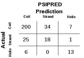
Finally, the matrix for PSIPRED:

There is less tendency to mispredict coil residues as helices, but, when compared to PHD, more tendency to mispredict coil as extended strand.

How should these three tools be compared?  It seems obvious at a glance that the results from PHD and PSIPRED are better than those from GOR4.  For secondary structure tools, it is common to report Q scores; these are accuracy scores that indicate the ratio of residues correctly predicted in a given category versus the number of residues that were observed in that category.  The following table shows the Q scores for the three categories, as well as an overall (total) Q score (the CEN column will be discussed momentarily):

When assessing secondary structure predictions, it is insufficient to look only at the Q_total score.  Why is that?  It is notable that TFPIα is 79% random coil.  A tool that blindly predicts ‘c’ for every residue would receive a very good Q_total score of 0.79, better than all three of these tools.  But that is an uninteresting prediction; we would need to consider all four of the scores when assessing these tools in order to correctly dismiss this hypothetical tool.

As I mentioned in the last post, it is often useful to have a single metric for comparing such classifiers.  Clearly, Q_total does not fit the bill, which corroborates my statement in the last post that “accuracy is a poor metric.”  One excellent metric for multi-class classifiers is “confusion entropy,” or CEN.  This technique accounts for every cell of the confusion matrix, measuring the entropy in the mispredictions in every row and in every column.  This provides a single number that is very representative of the overall predictive power.  The CEN scores range from 0 (indicating perfect classification) to 1 (indicating that every class was completely mispredicted evenly across all of the other possible classes).  The CEN calculation is described in Wei et al. (2010).  In this example, the CEN scores correlate well with the Q_total scores, but give the reviewer confidence that the failings of accuracy metrics are not an issue.

Another information theoretic approach, which accounts for “truth information completeness” and the “false information ratio,” is described in Holt et al. (2010).

References:

• Wei JM, Yuan XJ, Hu QH, and Wang SQ. 2010. A novel measure for evaluating classifiers. Expert Systems with Applications 37: 3799-3809.
• Holt RS, Mastromarino PA, Kao EK, and Hurley MB. 2010.  Information theoretic approach for performance evaluation of multi-class assignment systems.  Proc. of SPIE 7697: 76970R/1-12.

Metrics for Binary Classifiers: A Case Study

I have recently run across a few examples of classifiers in widely-used bioinformatics applications.  Assessing the ability of a classifier to provide good predictions is a difficult problem.  In this post and the next, I will describe the use of metrics in these applications, and how they might be improved.

Confusion Matrices

We will start with binary classification, in which samples are divided into two categories.  If we are testing individuals for the presence or absence of a disease, we can divide the samples into sets of individuals who have the disease (positives) and those that do not (negatives).  The classifier will attempt to divide the samples into the correct sets based on the results of testing.  Those who have the disease and are correctly identified as such by the classifier are true positives (TPs).  Those that do not have the disease and are correctly classified as such are known as true negatives (TNs).  Misclassifications are called false negatives (FNs) for subjects that have the disease but are classified as healthy, or false positives (FPs) for subjects that do not have the disease but are classified as diseased.

These can be arranged into a confusion matrix, as in the following:

It is common to use some of the following simple metrics, all based on the contents of the confusion matrix:

• precision, the fraction of positive results that are correct: TPs / (TPs + FPs)
• sensitivity (also called recall), the faction of positive subjects that are identified as positive: TPs / (TPs + FNs)
• specificity, the fraction of negative subjects that are identified as negative:  TNs / (FPs + TNs)
• accuracy, the ratio of correct classifications to the total number of samples: TPs + TNs / (TPs + TNs + FPs + FNs)

The relative importance of these metrics depends on the problem.  Is it useful to sacrifice specificity for sensitivity?  Is precision or specificity a better metric?  Are there useful metrics for directly comparing classifiers with a single number?

Case Study: Protein Domain Prediction

The prediction of protein domains based solely on the protein’s amino acid sequence is an important technique for functional annotation.  PROSITE, a database of protein families and domains on ExPASy, makes use of two types of approaches for detecting the presence of domains: patterns and profiles.  Each of the approaches is essentially an example of binary classification: a protein sequence is either predicted to have instances (one or more) of a particular domain, or it is predicted to have no instances of that domain.

In PROSITE, these classifiers are assessed by their precision and recall.  These metrics are widely used in information retrieval to assess the ability of a system to provide a list of relevant documents.  It is common to use an F-measure to summarize the two metrics by producing a harmonic mean of their values, but this score is not used in PROSITE.  Looking back at the equations for producing these values, it should be clear that the number of TNs is completely ignored; the ability of the system to correctly assess negatives is not considered.  Is this important?

We will look at Kunitz domains, a type of protein domain, as an illustrative example.  PROSITE includes two models for recognizing Kunitz domains: a pattern (PS00280) and a profile (PS50279). It is not obvious how many samples were in the overall set.  At the time of this writing, the models were assessed by their ability to classify the proteins in UniProtKB/SwissProt 2013_09, which contains 540958 samples.  This results in the following confusion matrices for the two classifiers:

The profile is clearly superior from a cursory glance, and this is reflected by the precision and recall metrics provided in PROSITE.  For the pattern, the precision is 0.9842 and the recall is 0.8432.  For the profile, the precision is 1.0 and the recall is 0.9948.

Accuracy is a Poor Metric

Accuracy is generally a poor metric, particularly when the samples are unbalanced (if, for example, there are far more negatives than positives, as is the case in this scenario).  The accuracy for the pattern is 0.9998835, and for the profile is 0.9999963.  It was wise to not provide accuracy scores, as they do not differentiate between the two classifiers very well.

Let’s consider what would have happened if there were far fewer TNs in the set of samples, which might have been the case if we filtered the input to not consider proteins that were very unlikely to include Kunitz domains.  If there were a total of 500 proteins considered, we would have ended up with 186 TNs for the pattern, and 189 TNs for the profile.  The accuracy would be 0.874 for the pattern, and 0.996 for the profile; the precision and recall metrics would remain unchanged.

Single Scores for Comparing Classifiers

While the precision and metric scores are useful, it can be difficult to compare classifiers using them.  Is it more important to ensure that most positive results are correct, that most positive subjects are identified as positive, or that most negative subjects are identified as negative?  Summarizing the performance of a classifier with a single number is a very useful feature.

• F-scores are measures that combine both precision and recall into a single number.  The F1 measure is the harmonic mean of these two numbers: (2 * precision * recall) / (precision + recall).  This formula can be modified to weigh these two numbers differently depending on their relative importance.  The result ranges from 1 (best case) down to 0 (worst case).
• The Matthews correlation coefficient (MCC) can be calculated from the confusion matrix using this formula: ((TPs * TNs) – (FPs * FNs)) / sqrt((TPs + FPs) * (TPs + FNs) * (TNs + FPs) * (TNs + FNs)).  This produces a number that indicates how well the predictions correlate to the actual observations.  The number ranges from 1 (best case) down to -1 (worst case), with a result of 0 indicating that the classifier performs no better than random guessing.

Of course, some amount of nuance is unavoidably lost when distilling the results of a classifier down to a single number.  However, such metrics can be extremely useful when comparing classifiers, and that appears to hold true for protein domain prediction.

Other Thoughts

It is notable that both the original metrics and my suggested metrics suffer from a more fundamental flaw.  It is common for a protein sequence to have multiple instances of a domain; if a profile or pattern recognizes one or more such domains without recognizing them all, it is still considered a “success.”  Thus, the metrics are really assessing how successful the classifiers are at establishing whether one or more domains exist in a protein, rather than how successful they are at identifying the location of every domain.  In the case of Kunitz domain prediction, the pattern results in 18 partial matches, and the profile results in 17 partial matches.

Fragment Recruitment Plotting in Python

I recently created a repository on GitHub for an application that I wrote a year and a half ago to generate fragment recruitment plots; it is located at https://github.com/mstrosaker/fragrecruit .  These plots are used in genomic and metagenomic analysis to visualize how short reads align to one or more reference genomes.  The application is written in Python, using matplotlib to generate the plots.

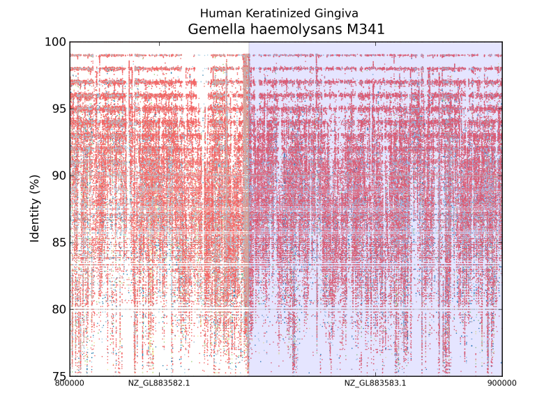
One such plot is shown below.  This plot shows the reads from human keratinized gingiva microbiome samples that align against a 100000bp section of the genome of a strain of the bacteria Gemella haemolysans.  Each sample is represented by a different color.  The sample sizes are dramatically different (reflecting differing depth of sequencing among the samples), which makes some colors much more predominant.  My application adds vertical lines to delineate the boundaries of contigs in the reference genome, and shades alternate contigs; as far as I know, it is the only application that identifies contigs along the reference genome in this manner.  It is interesting to note that, in some cases, fragments may tend to cluster near the edges of contigs; I suspect this is often due to the presence of repetitive sequences at the ends of contigs.

MQN Spaces for Drug Discovery: Part 5

Continued from part 4.

Conclusions

The simplicity of the MQN system belies its apparent ability to effectively represent structural characteristics of compounds that imply important bioactivities.  In order to obtain evidence of the utility of the system for drug discovery programs, this study assessed the potential of MQN representations to form the basis for predictive models and to estimate the structural diversity of chemical libraries.

Statistical analysis of the MQN descriptors for several sets of ligands established the presence of properties that serve to distinguish among the likely targets for the ligands.  The construction of classifiers trained on these ligands and tested with both ligands and decoys produced predictive models with accuracy that is competitive with models currently used in drug discovery.  It was further shown that transformation of the MQN space by dimensionality reduction techniques and kernel methods did not serve to improve the classification accuracy of the predictive models.  Among the categories of descriptors widely used in the construction of QSAR and QSPR models are constitutional descriptors, which provide structural details without consideration of topology or geometry; the results of this study suggest that MQNs can be useful when such descriptors are appropriate.

The rapid calculation of chemical diversity is an important aspect of chemical and fragment library construction.  Additionally, the ability of a representation to describe similarity without specifying the precise details of substructures has shown to be useful in scaffold hopping [1].  Comparisons of structural diversity calculations using MQNs with existing diversity calculation techniques based on fingerprint similarity show that an MQN-based approach produces results that are likely competitive, and possibly superior.  The discrete nature of the properties means that assessments of MQN-space consist primarily of integer calculations, without extensive requirements for more expensive floating point calculations.

Establishing the value of MQNs is significant because the computational intensity of many existing systems, which may perform expensive calculations of topological surface areas, pharmacophore fingerprints, and partition coefficients, prevents their widespread use on vast chemical spaces.  The speed of calculation for MQN properties make it a useful system for the fast assessment and classification of huge chemical spaces, as evidenced by its use in characterizing all of the 977 million compounds in the chemical universe database GDB-13 [2] and the 166.4 billion compounds in GDB-17 [3].  While speed is an important factor in such scenarios, the representation must also be rich enough to produce useful insights.  Though the MQN property space is limited by design to providing only constitutional descriptors, and the phenomenon of MQN isomers may produce difficulties yet to be characterized, this study provides evidence for its efficacy as a tool for cheminformatics tasks relevant to drug discovery.

References:

1. Böhm HJ, Flohr A, Stahl M.  2004.  Scaffold hopping.  Drug Discovery Today: Technologies 1(3): 217-224.
2. Blum LC, van Deursen R, and Reymond JL.  2011.  Visualisation and subsets of the chemical universe database GDB-13 for virtual screening.  J Comput Aided Mol Des 25(7): 637-647.
3. Ruddigkeit L, Blum LC, and Reymond JL. 2013. Visualization and virtual screening of the chemical universe database GDB-17. J Chem Inf Model 53(1): 56-65.

MQN Spaces for Drug Discovery: Part 4

Continued from part 3.

Third Hypothesis:

The calculation of diversity metrics from MQN properties provides diversity assessments that are comparable to those calculated from more complex (computationally intensive) sets of properties.

Methods

The multidimensional chemical space is reminiscent of search spaces in optimization problems.  In drug discovery, the processes of target and lead identification and lead optimization can be conceptualized as a search through the chemical space in order to find a compound that optimizes the search criteria (in terms of rule of 5 compliance, target affinity, and other criteria relevant to successful drugs).  Diversity metrics are widely employed when searching such search spaces in order to characterize the coverage of the space, and to ensure an appropriate balance between exploration of the overall search space and exploitation of specific promising regions.  Such diversity metrics were applied to the MQN representation of libraries to assess its ability to represent diversity in comparison to more complex systems of representation.

A common method for assessing the structural similarity of molecules is through the use of metrics to compare structural fingerprints.  Daylight fingerprints are an example of structural fingerprints used for this purpose; they are bit vectors that are constructed by hashing topological paths (along bonds) in the molecule.  The Tanimoto similarity coefficient is a popular method for comparing such fingerprints [1]; it is defined in the following equation, where a is the number of 1s in the first vector, b is the number of 1s in the second vector, and c is the number of positions in the two vectors that both contain 1s:

The Tanimoto similarity coefficient produces a number between 0 and 1, where 1 represents structurally identical molecules.  In order to be useful as a distance metric (where similar molecules should have low numbers, representing their closeness), the value of Ts should be subtracted from 1, producing the Tanimoto dissimilarity coefficient defined in the following equation:

As the Tanimoto coefficient is only useful for bit vectors, an alternative distance metric must be employed for vectors of MQNs.  Manhattan distance (also called city block distance) is often used for integral vectors like MQNs [2, 3]; it is simply the sum of the absolute differences between the values of the properties.

Diversity metrics have been widely employed to characterize populations in large search spaces in the field of evolutionary computation [4].  Four common diversity metrics were selected for purposes of comparison.  Each diversity calculation is normalized to the landscape diagonal (LD), which represents the distance across the entire landscape (all of the molecules in the data set).  This produces a number between 0 and 1, with a 1 indicating that the selected subset exhibits as much diversity as the entire set of molecules.

The mean of the distance between every member of the population and every other member is known to be a particularly effective metric, though it is computationally expensive (O(N^2), where N is the size of the population).  The calculation of the mean of the pairwise  distances, called PD, is defined by the following equation:

The greatest distance between any two members of the population is known as the diameter of the population, DP.  It is an intuitive metric, but is very susceptible to the presence of outliers.  The formula for calculating the diameter is defined by the following equation:

The distance between the mean of the population (also known as the center of gravity for the set of compounds) and the most distant member from the mean is the radius of the population, RP.  This approach can be modified to exclude extreme individuals as outliers.  The following equation shows the formula for calculating the radius:

The average of the distances from the mean of the population to every member of the population is referred to as DTAP, the distance to the average point.  This metric is defined by the following equation:

Diversity calculations from MQN representations (using a Manhattan distance metric) and Daylight fingerprint representations (using both Manhattan distance and Tanimoto dissimilarity coefficient metrics) were compared.  High correlation among the representations can provide evidence that their abilities to characterize diversity are comparable.

Results

The diversities of the ligands for each target were calculated, as well as the diversities of the overall set of all ligands.  As described in the methods, the diversities are normalized against the landscape diagonal, which is the longest extent of the hypercube containing all of the downloaded molecules (ligands and decoys).  The results of the diversity calculations are presented in the table on the right.  It is not surprising that the diversity as measured by DP and RP (the diameters and radii of the populations) is always notably higher than the diversity produced by the other metrics, as DP and RP are particularly prone to the influence of outliers.  In the case of RP, techniques have been developed to set aside the influence of extreme members of the population on the diversity [4]; such techniques were not explored in this study.

There is a very high correlation (Pearson’s correlation > 0.9) between the diversity measurements based on MQN properties and those based on fingerprints (using either Manhattan distances or Tanimoto coefficients as distance metrics).  This suggests that the representations produced by both systems tend to vary by roughly the same proportion in response to variability in the data.  It is interesting to note that the difference between diversities for larger sets in comparison to subsets is more substantial in the case of MQNs.  When considering the ratio of the diversities of the target classes to the diversity of all ligands, the correlation among the representation methods is only moderate (about 0.5).  This alone does not suggest that one method is  more capable of representing diversity, but it does indicate that more descriptive data concerning molecular structure may be encoded in the MQN system.

The group of ligands for GPB provides an illustrative example.  The use of Tanimoto coefficients with fingerprints indicates that this group represents over half of the structural diversity present in the entirety of the original set of ligands and decoys.  It does not seem likely that a library designer would find that assessment to be convincing.  In the case of the PD diversity metric, the use of MQN properties indicates that the ligands for GPB cover  only 8% of the structural diversity present in the overall set.

References:

1. Dean PM and Lewis RA, Eds.  2000.  Molecular Diversity in Drug Design.  Springer.  Print.
2. Reymond JL, Blum LC, and van Deursen R.  2011.  Exploring the chemical space of known and unknown organic small molecules at http://www.gdb.unibe.ch.  Chimia (Aarau) 65(11): 863-867.
3. van Deursen R, Blum LC, and Reymond JL.  2011.  Visualization of the chemical space of fragments, lead-like and drug-like molecules in PubChem.  J Comput Aided Mol Des 25: 649-662.
4. Corriveau G, Guilbault R, Tahan A, and Sabourin R.  2012.  Review and study of genotypic diversity measures for real-coded representations.  IEEE Transactions on Evolutionary Computation, 16(5):  695–710.

MQN Spaces for Drug Discovery: Part 3

Continued from part 2.

Second Hypothesis:

Effective models can be constructed to predict possible target families for novel small molecules based solely on MQN representations.

Methods

Classifiers were used to construct predictive models.  Ligands for the targets were used for the first six classes, and a seventh class consisting only of decoys was included to establish the ability to distinguish between compounds that exhibit activity with the various targets and those that do not exhibit activity for any of them.  Classifiers were constructed using the following approaches:

• classification and regression trees (CART);
• linear and quadratic discriminant analysis (LDA and QDA);
• support vector machines (SVMs); and
• neural networks (NNs).

These classifiers were implemented in the R statistical programming language.

The practice of reducing the dimensionality of the space via the identification of significant combinations of properties is widely employed to yield more effective classification.  The classifiers were applied both to untransformed data, and to data that were dimensionally reduced using the following techniques:

• PCA, using the top 3 and top 10 loadings;
• Kernel PCA based on a radial basis function (RBF) kernel;
• Classical metric multidimensional scaling (MDS);
• Kruskal’s non-metric MDS; and
• the weighted graph Laplacian (WGL), using the top 3 and 10 phis.

The efficacy of the classifiers was substantiated through the use of 5 x 2 cross-validation, in which multiple rounds of validation are performed with different partitions of the data, and the results are averaged across the rounds.  Both precision (the measure of how accurate the positive classifications are) and recall (the accuracy of the samples that should have been classified as positive) are important characteristics in such models.  These were calculated using the following equations, where tp is the number of true positives, fp is the number of false positives, and fn is the number of false negatives:

 

In order to provide a single metric for comparing predictive models, the F1 measure was used to provide a harmonic mean of precision and recall (assuming an equal importance in the two metrics), as defined in the following equation:

Results

Comparisons of the F1 measures for the various combinations of classifiers and input space transformations are shown in the following table:

Random guessing yields an F measure of 0.342, assuming the guesser knows the set sizes (which serves to reduce the impact of bias).  Among the evaluated classification approaches, CART provides the unique advantage of producing human-understandable decision trees; one such tree is presented in the following figure:

It is particularly interesting and perhaps unexpected that the various data transformation approaches did not produce gains in precision or recall in comparison to the untransformed data set.  The classifiers based on neural networks and support vector machines performed particularly well with the untransformed data, both yielding F measures over 0.9; the decision tree and linear discriminant analysis techniques both produced F measures exceeding 0.8.

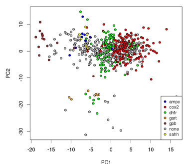
A plot of points corresponding to ligands for the various groups based on the first two principal components obtained from PCA is presented in the figure on the right.  These components account for 65.2% of the variability in the MQN properties among the targets.  Prior studies indicate that the first principal component is often reflective of the size of the molecules [1].  The first component in this analysis clearly includes large contributions from other properties; while the smaller GPB ligands tend to have low values for that component, the ligands for GART (which are the largest molecules on average) appear in the middle.  While finding the combinations of properties that result in the most variability is the goal of PCA, the first two components do not provide enough evidence to effectively separate the ligands.  It is clear from the results that even 10 components do not provide sufficiently separability for the classifiers.  This pattern is repeated for the other dimensionality reduction techniques, suggesting that such techniques are not effective for the development of classifiers for MQN-space.

Post-Mortem Comments

Reviewing this work in hindsight, there are a number of modifications I would have made to the methods.

The F1 metric is usually used in information retrieval scenarios, in which the true negative rate is less important.  As such, I would have used a different metric, such as the Matthews correlation coefficient, or a metric based on confusion entropy [2].

Rather than building 7-class classifiers, I would have used either binary classifiers (one for each target, proving the ability to differentiate among known ligands for a particular target and decoys for that target) or one-class classifiers (again, one for each target).  Such an approach would be more reflective of real-world analysis, in which one is interested in identifying the compounds that may exhibit activity with a target of interest.  I suspect this would have changed the conclusions with respect to data reduction methods, as PCA (or other techniques) would have readily identified the combinations of variables relevant to the specific target.

There are sometimes vast differences in the class sizes; these differences were not rigorously addressed.  A mixture of oversampling of minority classes and undersampling of majority classes was undertaken, depending on the class sizes.  The use of cross-validation may help to correct majority-class preferences that might have been introduced, but a method for sampling based on the imbalance ratio would have been useful to devise.

References:

1. Nguyen KT, Blum LC, van Deursen R, and Reymond JL.  2009.  Classification of organic molecules by molecular quantum numbers.  ChemMedChem 4(11): 1803-1805.
2. Wei JM, Yuan XJ, Hu QH, and Wang SQ.  2010.  A novel measure for evaluating classifiers.  Expert Systems with Applications 37: 3799-3809.

MQN Spaces for Drug Discovery: Part 2

Continued from part 1.

First Hypothesis:

Statistically significant differences can be identified between the properties of molecules that show affinity for major target families based solely on the MQN representations of the molecules.

Methods

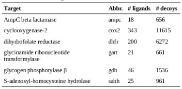
MQN-based assessments of large data sets have been shown to be practical, and so analysis for this study was limited to smaller sets.  A data set consisting of small molecules that have shown affinity for one or more targets among a collection of several target families was constructed.  Ligands and decoys (which are compounds that are chemically similar to known ligands but do not exhibit affinity for the targets) were downloaded from the Database of Useful Decoys (DUD) [1].  The set of targets was identified from those that were shown to cluster in MQN-space in prior literature [2], and are summarized in this table:

RDKit is an open source package for cheminformatics that provides programming interfaces for the in silico modeling and manipulation of molecules, and for measurement of their properties.  As RDKit does not accept the .mol2 file format used by ZINC and DUD as input, the Open Babel utility was used to convert .mol2 files to the SMILES (.smi) format [3].  RDKit was used to calculate the MQNs and other properties for the molecules that were chosen for analysis.

The goal of statistical testing is to analyze the differences between the means and variances of the properties of the ligands for each group, to establish if any such differences are significant.  Such differences provide for human-accessible descriptions of the qualities of the compounds that tend to provide affinity for one target family over another.

On the expectation that no underlying distribution can be assumed in the data, nonparametric tests were used exclusively.  Kruskal-Wallis one-way analysis of variance (ANOVA) was used to establish when a group has significant differences from the others, but does not identify which group or where the differences exist.  When statistically significant differences for MQN properties were confirmed with Kruskal-Wallis ANOVA, the Kruskal-Wallis signed rank test was further applied to pairwise comparisons of target groups to establish which groups exhibited significant differences.  In all cases, an alpha risk of 5 percent was used as the threshold, indicating that a null hypothesis can be rejected when the p-value is below 0.05.

Results

Ligands for each target were compared to the ligands for every other target, resulting in 6 choose 2 = 15 comparisons.  Statistical tests comparing each combination of targets for each property yielded numerous significant differences.  These differences are summarized in this figure:

Gray cells indicate that any measured difference between the ligand groups was not statistically significant for that property.  Other colors indicate an identified statistically-significant difference (p-value ≤ 0.05).  Dark blue indicates that the mean value was substantially higher for the first of the two compared groups; dark red indicates that the mean value was higher for the second.

There are numerous notable differences that can be identified from the heatmap; when necessary, such differences can be further visualized using histograms or boxplots.  Some interesting distinctions between the ligand groups include:

• AmpC and COX-2 ligands tend to include more acyclic tetravalent nodes than ligands for the other targets.
• COX-2 ligands are much more likely to include fluorine atoms, to have fewer hydrogen bond donors, and to include more cyclic divalent nodes than ligands for the other targets.
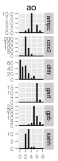
• DHFR ligands have fewer acyclic oxygen atoms on average in comparison to the other ligand groups; this is further explored with histograms below.
• GART and COX-2 ligands tend to have higher heavy atom counts, which is generally associated with higher molecular weights.  This is further detailed in the boxplot below.
• GPB ligands are much more likely to include cyclic oxygen atoms than ligands for the other targets.
• SAHH ligands are less likely to contain rings with 5 members than ligands for the other targets.

Histograms are useful for further exploration of the intuitions obtained during the analysis of discriminating features. As show in the figure on the left, the ligands for GART have a dramatic peak at a count of 6 acyclic oxygen atoms, while most DHFR ligands have 2 or fewer. The DHFR ligands are the only ones with a large proportion containing no acyclic oxygens.

Acyclic oxygens that are parts of amide, ketone, or sulfone moieties are notably prone to acting as hydrogen bond acceptors. However, acyclic ethers are significantly weaker acceptors than cyclic ethers [4]. While the presence of acyclic oxygens may suggest such H-bond activity, the MQN system is not capable of definitively distinguishing among the moieties.

The plot on the right clearly shows that the GART ligands have the highest mean number of heavy atoms, though COX-2 and DHFR ligands vary widely in size and can rival the size of GART ligands. AmpC, GPB, and SAHH ligands almost always contain fewer heavy atoms in comparison to GART ligands.

Naturally, the results of this form of analysis depend on the correctness and completeness of the data set.  If the analyzed ligands are not sufficiently representative of all the known ligands, or there are sizable quantities of unidentified ligands with different properties, then this approach may not successfully provide a good perspective on the archetypal ligand for a particular target.  However, it does provide a human-accessible method of assessing whether a novel compound fits the general known criteria for target affinity.  The availability of such distinguishing characteristics suggests that the construction of QSAR models for the prediction of biological activity may be fruitful.

References:

1. Huang N, Shoichet BK, and Irwin JJ.  2006.  Benchmarking sets for molecular docking.  J Med Chem 49(23): 6789–6801.
2. Nguyen KT, Blum LC, van Deursen R, and Reymond JL.  2009.  Classification of organic molecules by molecular quantum numbers.  ChemMedChem 4(11): 1803-1805.
3. O’Boyle NM, Banck M, James CA, Morley C, Vandermeersch T, Hutchison GR.  2011.  Open Babel: an open chemical toolbox.  Journal of Cheminformatics 3: 33.
4. Bissantz C, Kuhn B, and Stahl M.  2010.  A medicinal chemist’s guide to molecular interations.  J Med Chem 53(14): 5061-5084.

MQN Spaces for Drug Discovery: Part 1

This is the first of a series of posts based on a project that I devised and completed for a computational drug discovery course at the Johns Hopkins University.  The original submission was written in the style of an academic paper; the content has been modified, abridged, and rearranged to be more approachable as blog entries.  There are also some things that, in retrospect, I would have done differently if I were to revisit the project; the text is modified to note these new considerations.

The original title of the project was:

Assessment of the Utility of MQN Property Spaces for Drug Discovery

Abstract

The exploration and characterization of chemical space is an important enabling technology for drug discovery programs.  A system of Molecular Quantum Numbers (MQNs) has been proposed in which individual organic molecules are represented by a series of 42 integers, each of which is a count of a structural feature in the molecule.  This allows for the representation of compounds as points in a 42-dimensional property space.  While the clustering of compounds with similar structural and physiochemical properties has been observed in dimensionally-reduced MQN space, the ability to use this space for tasks of interest to drug discovery programs has not been well-characterized.  In this study, the predictive capabilities of the MQN representation system are assessed, as well as the ability of the system to represent true structural and physiochemical diversity in sets of compounds, which is useful for the development of focused libraries for compound or fragment screening.

Introduction and Objectives

Molecular Quantum Numbers (MQNs) provide the ability to represent molecules in a 42-dimensional property space [1]; the 42 MQNs are described in the table below.  Within this space, distance metrics can easily be used to quantify the similarity of compounds [2].  Dimensionality reduction methods are commonly employed to permit human visualization and interpretation of high-dimensional data sets; principal component analysis (PCA) is one such method that has been extensively applied to MQN data sets for this purpose [1-4].  These dimensionally-reduced property space maps can exhibit groupings of compounds with similar phsyiochemical and structural properties, and can even sometimes group compounds with similar bioactivities.

As these properties are generally reflective of molecular composition without consideration of topology or geometry, they fall into the category of constitutional descriptors in terms of quantitative structure-activity relationship (QSAR) analysis.  Notably missing from the MQN system are topological, steric, electrostatic, and other such useful and relevant properties of compounds; these properties include molecular volumes, topological polar surface areas, molar refractivities, partition coefficients, and many others.  Omission of such properties is partially due to the fact that they may not be easily quantizable, but more importantly, a single set of MQN properties can represent multiple molecules which may differ in such characteristics; molecules with the same set of MQNs are referred to as MQN isomers.  While this may be viewed as a representational limitation of the MQN system, it is indicated by the authors of the system that MQN isomers generally exhibit similar bioactivities [2].  It is possible that one MQN isomer could effectively bind to a drug target, while another has no such effects, though no such examples were found in a review of the literature.

An example of a molecule with its associated MQNs is presented in the figure below.  A major advantage of the MQN system is its simplicity: MQN properties can easily be manually established with basic knowledge of organic chemistry, mappings of the chemical space are more easily graspable by human observers, and large chemical spaces can be quickly assessed and classified due to the computational tractability [3].  While islands of molecules with affinities for certain targets have been observed in MQN property space [4] and simple diversity measurements have been described based on distances to the mathematical center of gravity of a set of compounds [3], the capabilities of the MQN approach for characterization of the chemical space in a manner useful for drug discovery are largely unproven.

I undertook a study to establish whether the representational power of the MQN system is sufficient for cheminformatics tasks that are relevant to drug discovery programs.  This objective is characterized by three hypotheses:

• Statistically significant differences can be identified between the properties of molecules that show affinity for major target families based solely on the MQN representations of the molecules.
• Effective models can be constructed to predict possible target families for novel small molecules based solely on MQN representations.
• The calculation of diversity metrics from MQN properties provides diversity assessments that are comparable to those calculated from more complex (computationally intensive) sets of properties.

The following three posts will each cover one of the objectives in further detail; conclusions will then be discussed in an additional post.

References:

1. Nguyen KT, Blum LC, van Deursen R, and Reymond JL.  2009.  Classification of organic molecules by molecular quantum numbers.  ChemMedChem 4(11): 1803-1805.
2. Reymond JL, Blum LC, and van Deursen R.  2011.  Exploring the chemical space of known and unknown organic small molecules at http://www.gdb.unibe.ch.  Chimia (Aarau) 65(11): 863-867.
3. van Deursen R, Blum LC, and Reymond JL.  2011.  Visualization of the chemical space of fragments, lead-like and drug-like molecules in PubChem.  J Comput Aided Mol Des 25: 649-662.
4. Reymond JL, van Deursen R, Blum LC, and Ruddigkeit L.  2010.  Chemical space as a source for new drugs.  Med Chem Commun 1: 30-38.